Runge–Kutta methods

In numerical analysis, the Runge–Kutta methods (German pronunciation: [ˌʁʊŋəˈkʊta]) are an important family of implicit and explicit iterative methods for the approximation of solutions of ordinary differential equations. These techniques were developed around 1900 by the German mathematicians C. Runge and M.W. Kutta.

See the article on numerical ordinary differential equations for more background and other methods. See also List of Runge–Kutta methods.

1 Common fourth-order Runge–Kutta method
2 Explicit Runge–Kutta methods
- 2.1 Examples
3 Usage
4 Adaptive Runge–Kutta methods
5 Implicit Runge–Kutta methods
- 5.1 Example
6 See also
7 References
8 External links

Common fourth-order Runge–Kutta method

One member of the family of Runge–Kutta methods is so commonly used that it is often referred to as "RK4", "classical Runge-Kutta method" or simply as "the Runge–Kutta method".

Let an initial value problem be specified as follows.

$y' = f(t, y), \quad y(t_0) = y_0$

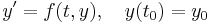
In words, what this means is that the rate at which y changes is a function of y and of t (time). At the start, time is $t_0$ and y is $y_0$ .

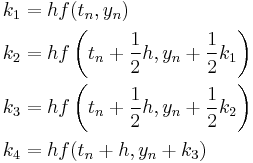
The RK4 method for this problem is given by the following equations:

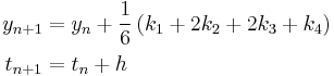
$\begin{align} y_{n%2B1} &= y_n %2B \frac{1}{6} \left(k_1 %2B 2k_2 %2B 2k_3 %2B k_4 \right) \\ t_{n%2B1} &= t_n %2B h \\ \end{align}$

where $y_{n%2B1}$ is the RK4 approximation of $y(t_{n%2B1})$ , and

$\begin{align} k_1 &= hf(t_n, y_n) \\ k_2 &= hf\left(t_n %2B \frac{1}{2}h , y_n %2B \frac{1}{2} k_1\right) \\ k_3 &= hf\left(t_n %2B \frac{1}{2}h , y_n %2B \frac{1}{2} k_2\right) \\ k_4 &= hf(t_n %2B h , y_n %2B k_3) \end{align}$

Thus, the next value ( $y_{n%2B1}$ ) is determined by the present value ( $y_n$ ) plus the weighted average of 4 deltas, where each delta is the product of the size of the interval ( $h = \Delta t$ ) and an estimated slope: $h \text{ } (slope) = h \text{ } f (t, \text{ } y) = \Delta t \text{ } (dy/dt) = \Delta y$ .

$k_1$ is the delta based on the slope at the beginning of the interval, using $y_n$ , ( Euler's method ) ;
$k_2$ is the delta based on the slope at the midpoint of the interval, using $y_n %2B$ 1/2 $k_1$ ;
$k_3$ is again the delta based on the slope at the midpoint, but now using $y_n %2B$ 1/2 $k_2$ ;
$k_4$ is the delta based on the slope at the end of the interval, using $y_n %2B k_3$ .

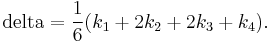
In averaging the four deltas, greater weight is given to the deltas at the midpoint:

$\mbox{delta} = \frac{1}{6}(k_1 %2B 2k_2 %2B 2k_3 %2B k_4).$

The RK4 method is a fourth-order method, meaning that the error per step is on the order of $h^5$ , while the total accumulated error has order $h^4$ .

Note that the above formulae are valid for both scalar- and vector-valued functions (i.e., $y$ can be a vector and $f$ an operator). For example one can integrate the time independent Schrödinger equation using the Hamiltonian operator as function $f$ .

Also note that if $f$ is independent of $y$ , so that the differential equation is equivalent to a simple integral, then RK4 is Simpson's rule.

Explicit Runge–Kutta methods

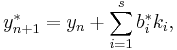
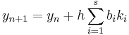
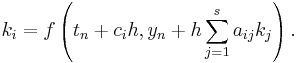
The family of explicit Runge–Kutta methods is a generalization of the RK4 method mentioned above. It is given by

$y_{n%2B1} = y_n %2B \sum_{i=1}^s b_i k_i,$

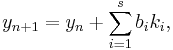
where

$k_1 = hf(t_n, y_n), \,$

$k_2 = hf(t_n%2Bc_2h, y_n%2Ba_{21}k_1), \,$

$k_3 = hf(t_n%2Bc_3h, y_n%2Ba_{31}k_1%2Ba_{32}k_2), \,$

$\vdots$

$k_s = hf(t_n%2Bc_sh, y_n%2Ba_{s1}k_1%2Ba_{s2}k_2%2B\cdots%2Ba_{s,s-1}k_{s-1}).$

(Note: the above equations have different but equivalent definitions in different texts).

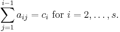
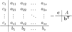
To specify a particular method, one needs to provide the integer s (the number of stages), and the coefficients a_ij (for 1 ≤ j < i ≤ s), b_i (for i = 1, 2, ..., s) and c_i (for i = 2, 3, ..., s). These data are usually arranged in a mnemonic device, known as a Butcher tableau (after John C. Butcher):

0
$c_2$	$a_{21}$
$c_3$	$a_{31}$	$a_{32}$
$\vdots$	$\vdots$		$\ddots$
$c_s$	$a_{s1}$	$a_{s2}$	$\cdots$	$a_{s,s-1}$
	$b_1$	$b_2$	$\cdots$	$b_{s-1}$	$b_s$

The Runge–Kutta method is consistent if

$\sum_{j=1}^{i-1} a_{ij} = c_i\ \mathrm{for}\ i=2, \ldots, s.$

There are also accompanying requirements if we require the method to have a certain order p, meaning that the local truncation error is O(h^p+1). These can be derived from the definition of the truncation error itself. For example, a 2-stage method has order 2 if b₁ + b₂ = 1, b₂c₂ = 1/2, and b₂a₂₁ = 1/2.

Examples

The RK4 method falls in this framework. Its tableau is:

0
1/2	1/2
1/2	0	1/2
1	0	0	1
	1/6	1/3	1/3	1/6

However, the simplest Runge–Kutta method is the (forward) Euler method, given by the formula 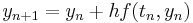$y_{n%2B1} = y_n %2B hf(t_n,y_n)$ . This is the only consistent explicit Runge–Kutta method with one stage. The corresponding tableau is:

	0
		1

An example of a second-order method with two stages is provided by the midpoint method

$y_{n%2B1} = y_n %2B hf\left(t_n%2B\frac{1}{2}h,y_n%2B\frac{1}{2}hf(t_n, y_n)\right).$

The corresponding tableau is:

0
1/2	1/2
	0	1

Note that this 'midpoint' method is not the optimal RK2 method. An alternative is provided by Heun's method, where the 1/2's in the tableau above are replaced by 1's and the b's row is [1/2, 1/2].

In fact, a family of RK2 methods is $y_{n%2B1} = y_n %2B h\bigl((1-\frac1{2\alpha})f \left( t, y_n \right) %2B \frac1{2\alpha}f \left( t %2B \alpha\,h, y_n %2B \alpha\,h f \left( t, y_n \right) \right)\bigr)$ where $\alpha=\frac12$ is the mid-point method and $\alpha=1$ is Heun's method.

If one wants to minimize the truncation error, the method below should be used (Atkinson p. 423). Other important methods are Fehlberg, Cash-Karp and Dormand-Prince. To use unequally spaced intervals requires an adaptive stepsize method.

Usage

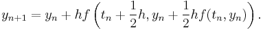
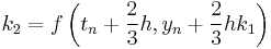
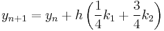
The following is an example usage of a two-stage explicit Runge–Kutta method:

0
2/3	2/3
	1/4	3/4

to solve the initial-value problem

$y' = \tan(y)%2B1,\quad y(1)=1,\ t\in [1, 1.1]$

with step size h=0.025.

The tableau above yields the equivalent corresponding equations below defining the method

$k_1 = f\left(t_n,y_n\right)$

$k_2 = f\left(t_n %2B \frac{2}{3}h, y_n %2B \frac{2}{3}h k_1\right)$

$y_{n%2B1} = y_n %2B h\left(\frac{1}{4}k_1%2B\frac{3}{4}k_2\right)$

$t_0=1$
	$y_0=1$
$t_1=1.025$
	$y_0 = 1$	$k_1=2.557407725$	$k_2 = f(t_0 %2B 2/3h ,y_0 %2B 2/3hk_1)$
	$y_1=y_0%2Bh(1/4k_1 %2B 3/4k_2)=1.066869388$
$t_2=1.05$
	$y_1 = 1.066869388$	$k_1=2.813524695$	$k_2 = f(t_1 %2B 2/3h, y_1 %2B 2/3hk_1)$
	$y_2=y_1%2Bh(1/4k_1 %2B 3/4k_2)=1.141332181$
$t_3=1.075$
	$y_2 = 1.141332181$	$k_1=3.183536647$	$k_2 = f(t_2 %2B 2/3h,y_2 %2B 2/3hk_1)$
	$y_3=y_2%2Bh(1/4k_1 %2B 3/4k_2)=1.227417567$
$t_4=1.1$
	$y_3 = 1.227417567$	$k_1=3.796866512$	$k_2 = f(t_3 %2B 2/3h,y_3 %2B 2/3hk_1)$
	$y_4=y_3%2Bh(1/4k_1 %2B 3/4k_2)=1.335079087$

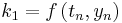
The numerical solutions correspond to the underlined values. Note that $f(t_i,k_1)$ has been calculated to avoid recalculation in the $y_i$ s.

Adaptive Runge–Kutta methods

The adaptive methods are designed to produce an estimate of the local truncation error of a single Runge–Kutta step. This is done by having two methods in the tableau, one with order $p$ and one with order $p - 1$ .

The lower-order step is given by

$y^*_{n%2B1} = y_n %2B \sum_{i=1}^s b^*_i k_i,$

where the $k_i$ are the same as for the higher order method. Then the error is

$e_{n%2B1} = y_{n%2B1} - y^*_{n%2B1} = h\sum_{i=1}^s (b_i - b^*_i) k_i,$

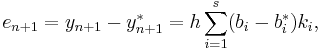
which is $O(h^p)$ . The Butcher Tableau for this kind of method is extended to give the values of $b^*_i$ :

0
$c_2$	$a_{21}$
$c_3$	$a_{31}$	$a_{32}$
$\vdots$	$\vdots$		$\ddots$
$c_s$	$a_{s1}$	$a_{s2}$	$\cdots$	$a_{s,s-1}$
	$b_1$	$b_2$	$\cdots$	$b_{s-1}$	$b_s$
	$b^*_1$	$b^*_2$	$\cdots$	$b^*_{s-1}$	$b^*_s$

The Runge–Kutta–Fehlberg method has two methods of orders 5 and 4. Its extended Butcher Tableau is:

0
1/4	1/4
3/8	3/32	9/32
12/13	1932/2197	−7200/2197	7296/2197
1	439/216	−8	3680/513	-845/4104
1/2	−8/27	2	−3544/2565	1859/4104	−11/40
	16/135	0	6656/12825	28561/56430	−9/50	2/55
	25/216	0	1408/2565	2197/4104	−1/5	0

However, the simplest adaptive Runge–Kutta method involves combining the Heun method, which is order 2, with the Euler method, which is order 1. Its extended Butcher Tableau is:

0
1	1
	1/2	1/2
	1	0

The error estimate is used to control the stepsize.

Other adaptive Runge–Kutta methods are the Bogacki–Shampine method (orders 3 and 2), the Cash–Karp method and the Dormand–Prince method (both with orders 5 and 4).

Implicit Runge–Kutta methods

The implicit methods are more general than the explicit ones. The distinction shows up in the Butcher Tableau: for an implicit method, the coefficient matrix $a_{ij}$ is not necessarily lower triangular:

$\begin{array}{c|cccc} c_1 & a_{11} & a_{12}& \dots & a_{1s}\\ c_2 & a_{21} & a_{22}& \dots & a_{2s}\\ \vdots & \vdots & \vdots& \ddots& \vdots\\ c_s & a_{s1} & a_{s2}& \dots & a_{ss} \\ \hline & b_1 & b_2 & \dots & b_s\\ \end{array} = \begin{array}{c|c} \mathbf{c}& A\\ \hline & \mathbf{b^T} \\ \end{array}$

The approximate solution to the initial value problem reflects the greater number of coefficients:

$y_{n%2B1} = y_n %2B h \sum_{i=1}^s b_i k_i\,$

$k_i = f\left(t_n %2B c_i h, y_n %2B h \sum_{j = 1}^s a_{ij} k_j\right).$

Due to the fullness of the matrix $a_{ij}$ , the evaluation of each $k_i$ is now considerably involved and dependent on the specific function $f(t, y)$ . Despite the difficulties, implicit methods are of great importance due to their high (possibly unconditional) stability, which is especially important in the solution of partial differential equations. The simplest example of an implicit Runge–Kutta method is the backward Euler method:

$y_{n %2B 1} = y_n %2B h f(t_n %2B h, y_{n %2B 1})\,$

The Butcher Tableau for this is simply:

$\begin{array}{c|c} 1 & 1 \\ \hline & 1 \\ \end{array}$

It can be difficult to make sense of even this simple implicit method, as seen from the expression for $k_1$ :

$k_1 = f(t_n %2B c_1 h, y_n %2B h a_{11} k_1) \rightarrow k_1 = f(t_n %2B h, y_n %2B h k_1).$

In this case, the awkward expression above can be simplified by noting that

$y_{n%2B1} = y_n %2B h k_1 \rightarrow h k_1 = y_{n%2B1} - y_n\,$

so that

$k_1 = f(t_n %2B h, y_n %2B y_{n%2B1} - y_n) = f(t_n %2B h, y_{n%2B1}).\,$

from which

$y_{n %2B 1} = y_n %2B h f(t_n %2B h, y_{n %2B 1})\,$

follows. Though simpler than the "raw" representation before manipulation, this is an implicit relation so that the actual solution is problem dependent. Multistep implicit methods have been used with success by some researchers. The combination of stability, higher order accuracy with fewer steps, and stepping that depends only on the previous value makes them attractive; however the complicated problem-specific implementation and the fact that $k_i$ must often be approximated iteratively means that they are not common.

Example

Another example for an implicit Runge-Kutta method is the Crank–Nicolson method, also known as the trapezoid method. Its Butcher Tableau is:

$\begin{array}{c|cc} 0 & 0& 0\\ 1 & \frac{1}{2}& \frac{1}{2}\\ \hline & \frac{1}{2}&\frac{1}{2}\\ \end{array}$

References

John C. Butcher (2003). Numerical methods for ordinary differential equations. John Wiley & Sons. ISBN 0471967580.
George E. Forsythe, Michael A. Malcolm, and Cleve B. Moler (1977). Computer Methods for Mathematical Computations. Prentice-Hall. (see Chapter 6).
Ernst Hairer, Syvert Paul Nørsett, and Gerhard Wanner (1993). Solving ordinary differential equations I: Nonstiff problems (2nd ed.). Springer Verlag. ISBN 3-540-56670-8.

Press, WH; Teukolsky, SA; Vetterling, WT; Flannery, BP (2007). "Section 17.1 Runge-Kutta Method". Numerical Recipes: The Art of Scientific Computing (3rd ed.). New York: Cambridge University Press. ISBN 978-0-521-88068-8. http://apps.nrbook.com/empanel/index.html#pg=907. . Also, Section 17.2. Adaptive Stepsize Control for Runge-Kutta.

Autar Kaw, Egwu Kalu (2008). Numerical Methods with Applications (1st ed.). autarkaw.com. http://numericalmethods.eng.usf.edu/topics/textbook_index.html.
Kendall E. Atkinson (1989). An Introduction to Numerical Analysis. John Wiley & Sons.
F. Cellier, E. Kofman (2006). Continuous System Simulation. Springer Verlag. ISBN 0-387-26102-8.

External links

Runge–Kutta 4th Order Method
Runge Kutta Method for O.D.E.'s
DotNumerics: Ordinary Differential Equations for C# and VB.NET – Initial-value problem for nonstiff and stiff ordinary differential equations (explicit Runge-Kutta, implicit Runge-Kutta, Gear's BDF and Adams-Moulton).
GafferOnGames – A physics resource for computer programmers
PottersWheel – Parameter calibration in ODE systems using implicit Runge-Kutta integration

Numerical integration

First order methods	Euler method · Backward Euler · Semi-implicit Euler · Exponential Euler

Second order methods	Verlet integration · Velocity Verlet · Crank–Nicolson method · Beeman's algorithm · Midpoint method · Heun's method · Newmark-beta method · Leapfrog integration

Higher order methods	Runge–Kutta methods · List of Runge–Kutta methods · Linear multistep method